Thierry Warin, PhD: [R Course] Random Forest

Thierry Warin

doi:10.6084/m9.figshare.11842416.v2

Introduction

The Random Forest estimator can be used for classification as well as for regression. Random forests are a type of tree ensemble technique that works by building a large number of decision trees from significantly modified versions of the training set (Breiman 2001a). The ensemble is comprised of this collection of trees. Each ensemble member produces a different prediction when a new sample is predicted. These are then averaged to get the ensemble forecast for the new data point.

Random forest models are extremely strong and can accurately replicate the underlying data patterns. While this model is computationally demanding, it is extremely low-maintenance, requiring very little preparation (as documented in Appendix A).

We can use the ranger package to fit a random forest model to the training data using the same predictor set as the linear model (without doing any additional preprocessing steps). This model requires no preprocessing, allowing for the application of a straightforward formula.

We will use the Netflix dataset, see below.

EDA

As a first step in modeling, it’s always a good idea to explore the variables in the dataset.

if(!require(devtools)) install.packages("devtools")
devtools::install_github("kassambara/factoextra")
if(!require(FactoMineR)) install.packages("FactoMineR")
if(!require(tidymodels)) install.packages("tidymodels")
if(!require(caret)) install.packages("caret")

library(tidyverse)
movies <- readr::read_csv("https://www.warin.ca/datalake/courses_data/qmibr/session9/movies_metadata.csv")
df <- movies %>%
  # select features
  select(budget, popularity, revenue, runtime, vote_average, vote_count)

Let us remove the Nas:

df <- na.omit(df)
head(df)

# A tibble: 6 × 6
    budget popularity   revenue runtime vote_average vote_count
     <dbl>      <dbl>     <dbl>   <dbl>        <dbl>      <dbl>
1 30000000      21.9  373554033      81          7.7       5415
2 65000000      17.0  262797249     104          6.9       2413
3        0      11.7          0     101          6.5         92
4 16000000       3.86  81452156     127          6.1         34
5        0       8.39  76578911     106          5.7        173
6 60000000      17.9  187436818     170          7.7       1886

Random Forest for Regression

One risk associated with machine learning is that the computer learns too much from our sample data and hence becomes less reliable during real-world testing. This is referred to as overtraining or overfitting. This issue is resolved by dividing the dataset into training and testing sets. The training set is used to train the model, whereas the test set is used to estimate the model’s performance on new or unstructured data.

The division is based on ratios, and the most often used ratios are 80/20, 75/25, or 7/30, with the training data receiving a greater share of the dataset and the test data receiving the remaining tiny amount.

The rsample package’s initial split function is used to divide the dataset into training and testing sets. We collect the data that will be divided and the proportion that will act as the cutoff for the two sets.

library(tidymodels)
# Fix the random numbers by setting the seed 
# This enables the analysis to be reproducible when random numbers are used 
set.seed(222)
# Put 3/4 of the data into the training set 
data_split <- initial_split(df, prop = 3/4)

# Create data frames for the two sets:
train_data <- training(data_split)
test_data  <- testing(data_split)

We can define the model with specific parameters:

 tidymodels_prefer()

lr_model <- 
  # specify that the model is a random forest
  linear_reg() %>%
  # select the engine/package that underlies the model
  set_engine("lm") %>%
  # choose either the continuous regression or binary classification mode
  set_mode("regression")

# create CV object from training data
folds <- vfold_cv(train_data, v = 2)

The recipes package (Kuhn and Wickham 2020a) defines a recipe object that will be used to model variables and perform variable preprocessing. Recipe(), prep(), juice(), and bake() are the four primary functions (). recipe() specifies the operations that will be performed on the data and their related responsibilities. After defining the preprocessing processes, any parameters are calculated using prep ().

Manually constructed recipes can be developed by successively assigning responsibilities to variables in a data collection. To begin, we’ll generate a recipe object using the train set data, describe the processing steps, and then transform the data using step_*. We prepare the recipe after it is complete. For instance, to generate a basic recipe consisting just of an outcome and predictors, normalise the predictors, and impute missing values in the predictors:

# define the recipe
train_data_recipe <- 
  recipe(popularity ~ ., 
         data = df)
  
  # and some pre-processing steps
#  %>% step_normalize(all_numeric()) %>%
#  step_knnimpute(all_predictors())

The model is specified using the parsnip package (Kuhn and Vaughan 2020a). This package provides a clean, uniform interface to models for a variety of models without delving into the syntactical details of the underlying packages. The parsnip bundle assists us in defining:

- the type of model e.g random forest,
- the mode of the model whether is regression or classification
- the computational engine is the name of the R package.

rf_model <- 
  # specify that the model is a random forest
  rand_forest() %>%
  # specify that the `mtry` parameter needs to be tuned
  set_args(mtry = tune()) %>%
  # select the engine/package that underlies the model
  set_engine("ranger", importance = "impurity") %>%
  # choose either the continuous regression or binary classification mode
  set_mode("regression")

# set the workflow
rf_workflow <- workflow() %>%
  # add the recipe
  add_recipe(train_data_recipe) %>%
  # add the model
  add_model(rf_model)

Tune the parameters

# specify which values you want to try with CV
rf_grid <- expand.grid(mtry = c(3, 4, 5))
# extract results
rf_tune_results <- rf_workflow %>%
  tune_grid(resamples = folds, #CV object
            grid = rf_grid, # grid of values to try
            metrics = metric_set(rmse) # metrics we care about
            )

# print results
rf_tune_results %>%
  collect_metrics()

# A tibble: 3 × 7
   mtry .metric .estimator  mean     n std_err .config             
  <dbl> <chr>   <chr>      <dbl> <int>   <dbl> <chr>               
1     3 rmse    standard    5.03     2   0.717 Preprocessor1_Model1
2     4 rmse    standard    5.07     2   0.683 Preprocessor1_Model2
3     5 rmse    standard    5.12     2   0.634 Preprocessor1_Model3

param_final <- rf_tune_results %>%
  select_best(metric = "rmse")
param_final

# A tibble: 1 × 2
   mtry .config             
  <dbl> <chr>               
1     3 Preprocessor1_Model1

rf_workflow <- rf_workflow %>%
  finalize_workflow(param_final)

test_data

After specifying the model type, engine, and mode, the fit function may be used to train the model. We just parse the requested model and the modified training set from the prepared recipe into the fit.

rf_fit <- rf_workflow %>%
  # fit on the training set and evaluate on test set
  last_fit(data_split)

rf_fit

# Resampling results
# Manual resampling 
# A tibble: 1 × 6
  splits                id              .metrics .notes   .predictions
  <list>                <chr>           <list>   <list>   <list>      
1 <split [33902/11301]> train/test spl… <tibble> <tibble> <tibble>    
# … with 1 more variable: .workflow <list>

test_performance <- rf_fit %>% collect_metrics()
test_performance

# A tibble: 2 × 4
  .metric .estimator .estimate .config             
  <chr>   <chr>          <dbl> <chr>               
1 rmse    standard       3.74  Preprocessor1_Model1
2 rsq     standard       0.514 Preprocessor1_Model1

# generate predictions from the test set
test_predictions <- rf_fit %>% collect_predictions()
test_predictions

# A tibble: 11,301 × 5
   id               .pred  .row popularity .config             
   <chr>            <dbl> <int>      <dbl> <chr>               
 1 train/test split  9.22     7       6.68 Preprocessor1_Model1
 2 train/test split  8.40    12       5.43 Preprocessor1_Model1
 3 train/test split  8.83    15       7.28 Preprocessor1_Model1
 4 train/test split  9.39    17      10.7  Preprocessor1_Model1
 5 train/test split  9.94    20       7.34 Preprocessor1_Model1
 6 train/test split  8.14    22      10.7  Preprocessor1_Model1
 7 train/test split  8.48    24      12.1  Preprocessor1_Model1
 8 train/test split  3.60    28       2.23 Preprocessor1_Model1
 9 train/test split  3.02    30       1.10 Preprocessor1_Model1
10 train/test split 11.6     34      14.4  Preprocessor1_Model1
# … with 11,291 more rows

# generate a confusion matrix
test_predictions %>% 
  metrics(truth = popularity, estimate = .pred)

# A tibble: 3 × 3
  .metric .estimator .estimate
  <chr>   <chr>          <dbl>
1 rmse    standard       3.74 
2 rsq     standard       0.514
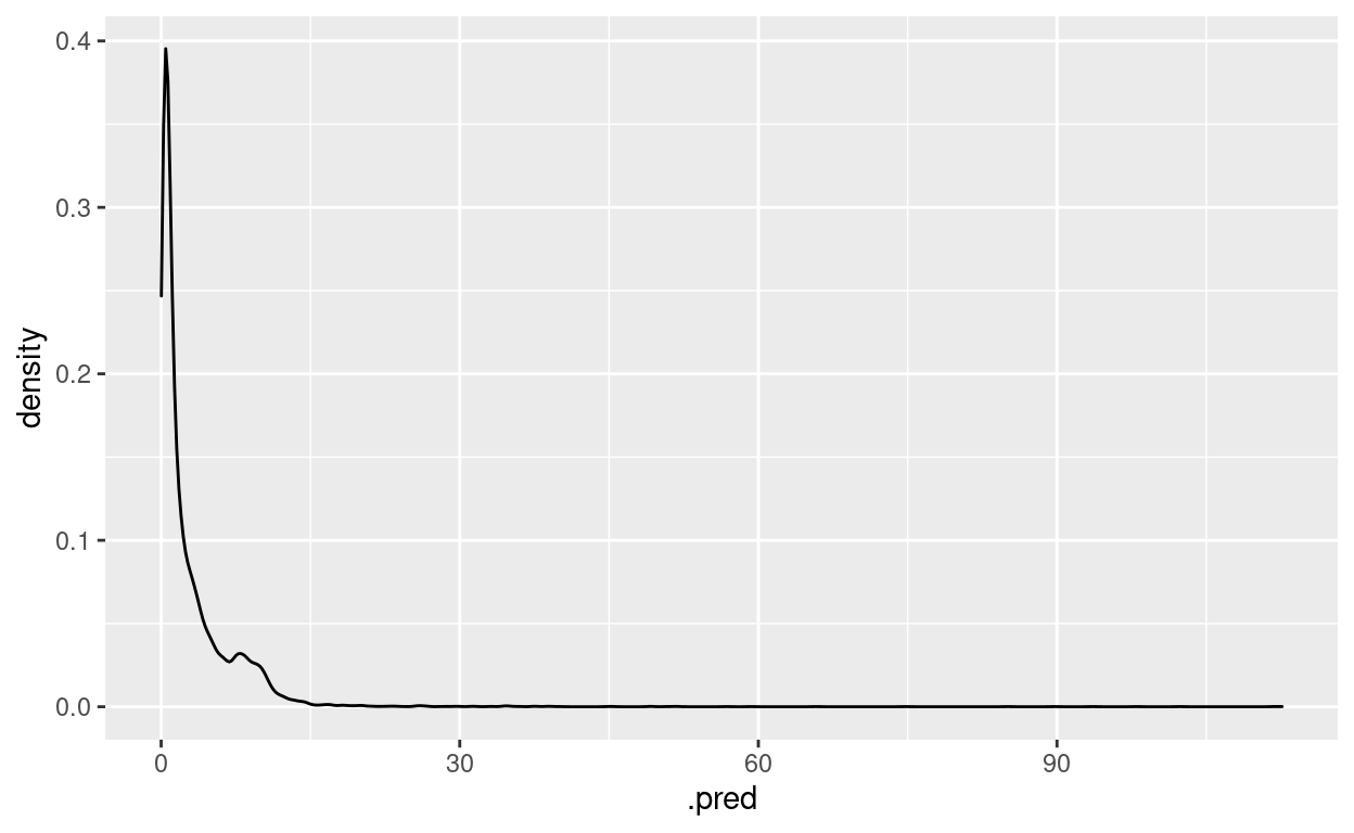
3 mae     standard       1.24

test_predictions %>%
  ggplot() +
  geom_density(aes(x = .pred, fill = popularity), 
               alpha = 0.5)

test_predictions <- rf_fit %>% pull(.predictions)
test_predictions

[[1]]
# A tibble: 11,301 × 4
   .pred  .row popularity .config             
   <dbl> <int>      <dbl> <chr>               
 1  9.22     7       6.68 Preprocessor1_Model1
 2  8.40    12       5.43 Preprocessor1_Model1
 3  8.83    15       7.28 Preprocessor1_Model1
 4  9.39    17      10.7  Preprocessor1_Model1
 5  9.94    20       7.34 Preprocessor1_Model1
 6  8.14    22      10.7  Preprocessor1_Model1
 7  8.48    24      12.1  Preprocessor1_Model1
 8  3.60    28       2.23 Preprocessor1_Model1
 9  3.02    30       1.10 Preprocessor1_Model1
10 11.6     34      14.4  Preprocessor1_Model1
# … with 11,291 more rows

Fitting and using your final model

final_model <- fit(rf_workflow, df)
final_model

══ Workflow [trained] ════════════════════════════════════════════════
Preprocessor: Recipe
Model: rand_forest()

── Preprocessor ──────────────────────────────────────────────────────
0 Recipe Steps

── Model ─────────────────────────────────────────────────────────────
Ranger result

Call:
 ranger::ranger(x = maybe_data_frame(x), y = y, mtry = min_cols(~3,      x), importance = ~"impurity", num.threads = 1, verbose = FALSE,      seed = sample.int(10^5, 1)) 

Type:                             Regression 
Number of trees:                  500 
Sample size:                      45203 
Number of independent variables:  5 
Mtry:                             3 
Target node size:                 5 
Variable importance mode:         impurity 
Splitrule:                        variance 
OOB prediction error (MSE):       22.28497 
R squared (OOB):                  0.3848619

Example of a new prediction:

new_obs <- tribble(~budget, ~revenue, ~runtime, ~vote_average, ~vote_count,
                     200000000, 300000000, 90, 7.7, 5145)
new_obs

# A tibble: 1 × 5
     budget   revenue runtime vote_average vote_count
      <dbl>     <dbl>   <dbl>        <dbl>      <dbl>
1 200000000 300000000      90          7.7       5145

predict(final_model, new_data = new_obs)

# A tibble: 1 × 1
  .pred
  <dbl>
1  35.6

Variable importance:

ranger_obj <- pull_workflow_fit(final_model)$fit
ranger_obj

Ranger result

Call:
 ranger::ranger(x = maybe_data_frame(x), y = y, mtry = min_cols(~3,      x), importance = ~"impurity", num.threads = 1, verbose = FALSE,      seed = sample.int(10^5, 1)) 

Type:                             Regression 
Number of trees:                  500 
Sample size:                      45203 
Number of independent variables:  5 
Mtry:                             3 
Target node size:                 5 
Variable importance mode:         impurity 
Splitrule:                        variance 
OOB prediction error (MSE):       22.28497 
R squared (OOB):                  0.3848619

ranger_obj$variable.importance

      budget      revenue      runtime vote_average   vote_count 
    157501.0     355529.6     117058.3     127223.3     748104.0

Random Forest for Classification

train_data

 tidymodels_prefer()

df_clean <- df %>% mutate(pop_class = case_when(popularity > 0.5 ~ "up", TRUE ~ "down"))
df_clean$popularity <- NULL
df_clean$pop_class <- as.factor(df_clean$pop_class)

library(tidymodels)
# Fix the random numbers by setting the seed 
# This enables the analysis to be reproducible when random numbers are used 
set.seed(222)
# Put 3/4 of the data into the training set 
data_split <- initial_split(df_clean, prop = 3/4)

# Create data frames for the two sets:
train_data <- training(data_split)
test_data  <- testing(data_split)

# create CV object from training data
folds <- vfold_cv(train_data, v = 2)

For instance, if we want to fit a random forest model as implemented by the ranger package for the purpose of classification and we want to tune the mtry parameter (the number of randomly selected variables to be considered at each split in the trees), then we would define the following model specification:

# define the recipe
train_data_recipe <- 
  recipe(pop_class ~ ., 
         data = df_clean)
  
  # and some pre-processing steps
#  %>% step_normalize(all_numeric()) %>%
#  step_knnimpute(all_predictors())

rf_model <- 
  # specify that the model is a random forest
  rand_forest() %>%
  # specify that the `mtry` parameter needs to be tuned
  set_args(mtry = tune()) %>%
  # select the engine/package that underlies the model
  set_engine("ranger", importance = "impurity") %>%
  # choose either the continuous regression or binary classification mode
  set_mode("classification")

# set the workflow
rf_workflow <- workflow() %>%
  # add the recipe
  add_recipe(train_data_recipe) %>%
  # add the model
  add_model(rf_model)

Tune the parameters

# specify which values you want to try with CV
rf_grid <- expand.grid(mtry = c(3, 4, 5))
# extract results
rf_tune_results <- rf_workflow %>%
  tune_grid(resamples = folds, #CV object
            grid = rf_grid, # grid of values to try
            metrics = metric_set(accuracy, roc_auc) # metrics we care about
            )

# print results
rf_tune_results %>%
  collect_metrics()

# A tibble: 6 × 7
   mtry .metric  .estimator  mean     n  std_err .config             
  <dbl> <chr>    <chr>      <dbl> <int>    <dbl> <chr>               
1     3 accuracy binary     0.850     2 0.000678 Preprocessor1_Model1
2     3 roc_auc  binary     0.922     2 0.000481 Preprocessor1_Model1
3     4 accuracy binary     0.846     2 0.000206 Preprocessor1_Model2
4     4 roc_auc  binary     0.918     2 0.000639 Preprocessor1_Model2
5     5 accuracy binary     0.844     2 0.000295 Preprocessor1_Model3
6     5 roc_auc  binary     0.917     2 0.000681 Preprocessor1_Model3

mtry = 3 is the best

Let’s confirm it automatically:

param_final <- rf_tune_results %>%
  select_best(metric = "accuracy")
param_final

# A tibble: 1 × 2
   mtry .config             
  <dbl> <chr>               
1     3 Preprocessor1_Model1

rf_workflow <- rf_workflow %>%
  finalize_workflow(param_final)

test_data

rf_fit <- rf_workflow %>%
  # fit on the training set and evaluate on test set
  last_fit(data_split)

rf_fit

# Resampling results
# Manual resampling 
# A tibble: 1 × 6
  splits                id              .metrics .notes   .predictions
  <list>                <chr>           <list>   <list>   <list>      
1 <split [33902/11301]> train/test spl… <tibble> <tibble> <tibble>    
# … with 1 more variable: .workflow <list>

test_performance <- rf_fit %>% collect_metrics()
test_performance

# A tibble: 2 × 4
  .metric  .estimator .estimate .config             
  <chr>    <chr>          <dbl> <chr>               
1 accuracy binary         0.854 Preprocessor1_Model1
2 roc_auc  binary         0.924 Preprocessor1_Model1

# generate predictions from the test set
test_predictions <- rf_fit %>% collect_predictions()
test_predictions

# A tibble: 11,301 × 7
   id          .pred_down .pred_up  .row .pred_class pop_class .config
   <chr>            <dbl>    <dbl> <int> <fct>       <fct>     <chr>  
 1 train/test…   0.0168      0.983     7 up          up        Prepro…
 2 train/test…   0.000222    1.00     12 up          up        Prepro…
 3 train/test…   0.0111      0.989    15 up          up        Prepro…
 4 train/test…   0           1        17 up          up        Prepro…
 5 train/test…   0           1        20 up          up        Prepro…
 6 train/test…   0           1        22 up          up        Prepro…
 7 train/test…   0           1        24 up          up        Prepro…
 8 train/test…   0           1        28 up          up        Prepro…
 9 train/test…   0.000133    1.00     30 up          up        Prepro…
10 train/test…   0           1        34 up          up        Prepro…
# … with 11,291 more rows

# generate a confusion matrix
test_predictions %>% 
  conf_mat(truth = pop_class, estimate = .pred_class)

          Truth
Prediction down   up
      down 2601  908
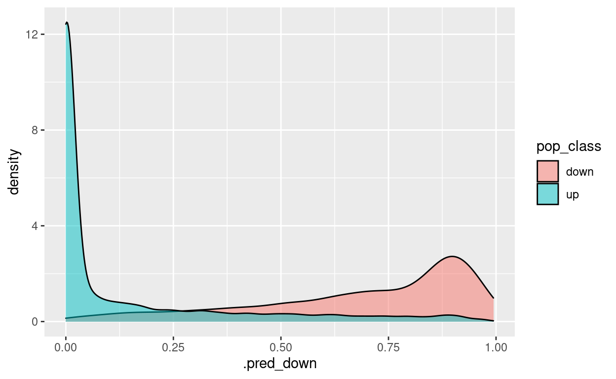
      up    742 7050

test_predictions %>%
  ggplot() +
  geom_density(aes(x = .pred_down, fill = pop_class), 
               alpha = 0.5)

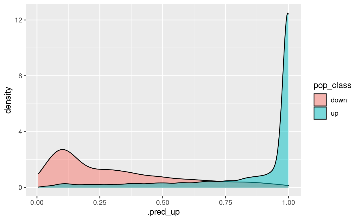
test_predictions %>%
  ggplot() +
  geom_density(aes(x = .pred_up, fill = pop_class), 
               alpha = 0.5)

test_predictions <- rf_fit %>% pull(.predictions)
test_predictions

[[1]]
# A tibble: 11,301 × 6
   .pred_down .pred_up  .row .pred_class pop_class .config            
        <dbl>    <dbl> <int> <fct>       <fct>     <chr>              
 1   0.0168      0.983     7 up          up        Preprocessor1_Mode…
 2   0.000222    1.00     12 up          up        Preprocessor1_Mode…
 3   0.0111      0.989    15 up          up        Preprocessor1_Mode…
 4   0           1        17 up          up        Preprocessor1_Mode…
 5   0           1        20 up          up        Preprocessor1_Mode…
 6   0           1        22 up          up        Preprocessor1_Mode…
 7   0           1        24 up          up        Preprocessor1_Mode…
 8   0           1        28 up          up        Preprocessor1_Mode…
 9   0.000133    1.00     30 up          up        Preprocessor1_Mode…
10   0           1        34 up          up        Preprocessor1_Mode…
# … with 11,291 more rows

Fitting and using your final model

final_model <- fit(rf_workflow, df_clean)
final_model

══ Workflow [trained] ════════════════════════════════════════════════
Preprocessor: Recipe
Model: rand_forest()

── Preprocessor ──────────────────────────────────────────────────────
0 Recipe Steps

── Model ─────────────────────────────────────────────────────────────
Ranger result

Call:
 ranger::ranger(x = maybe_data_frame(x), y = y, mtry = min_cols(~3,      x), importance = ~"impurity", num.threads = 1, verbose = FALSE,      seed = sample.int(10^5, 1), probability = TRUE) 

Type:                             Probability estimation 
Number of trees:                  500 
Sample size:                      45203 
Number of independent variables:  5 
Mtry:                             3 
Target node size:                 10 
Variable importance mode:         impurity 
Splitrule:                        gini 
OOB prediction error (Brier s.):  0.1018599

Example of a new prediction:

new_obs <- tribble(~budget, ~revenue, ~runtime, ~vote_average, ~vote_count,
                     200000000, 300000000, 90, 7.7, 5145)
new_obs

# A tibble: 1 × 5
     budget   revenue runtime vote_average vote_count
      <dbl>     <dbl>   <dbl>        <dbl>      <dbl>
1 200000000 300000000      90          7.7       5145

predict(final_model, new_data = new_obs)

# A tibble: 1 × 1
  .pred_class
  <fct>      
1 up

Variable importance:

ranger_obj <- pull_workflow_fit(final_model)$fit
ranger_obj

Ranger result

Call:
 ranger::ranger(x = maybe_data_frame(x), y = y, mtry = min_cols(~3,      x), importance = ~"impurity", num.threads = 1, verbose = FALSE,      seed = sample.int(10^5, 1), probability = TRUE) 

Type:                             Probability estimation 
Number of trees:                  500 
Sample size:                      45203 
Number of independent variables:  5 
Mtry:                             3 
Target node size:                 10 
Variable importance mode:         impurity 
Splitrule:                        gini 
OOB prediction error (Brier s.):  0.1018599

ranger_obj$variable.importance

      budget      revenue      runtime vote_average   vote_count 
    404.9120     196.9721    1773.7982    2123.4885    8998.1306

[R Course] Random Forest

Introduction

EDA

Random Forest for Regression

Tune the parameters

test_data

Fitting and using your final model

Random Forest for Classification

train_data

Tune the parameters

test_data

Fitting and using your final model

References

Citation