Nüance-R has made available the Distill package (Allaire, Iannone, and Xie 2018) for you to use it. Distill ships with a CSS framework and a collection of custom web components that make building interactive academic articles easier.
Creating an article
To create a Distill article follow the steps:
File > New File > R Markdown...
The following window will open.
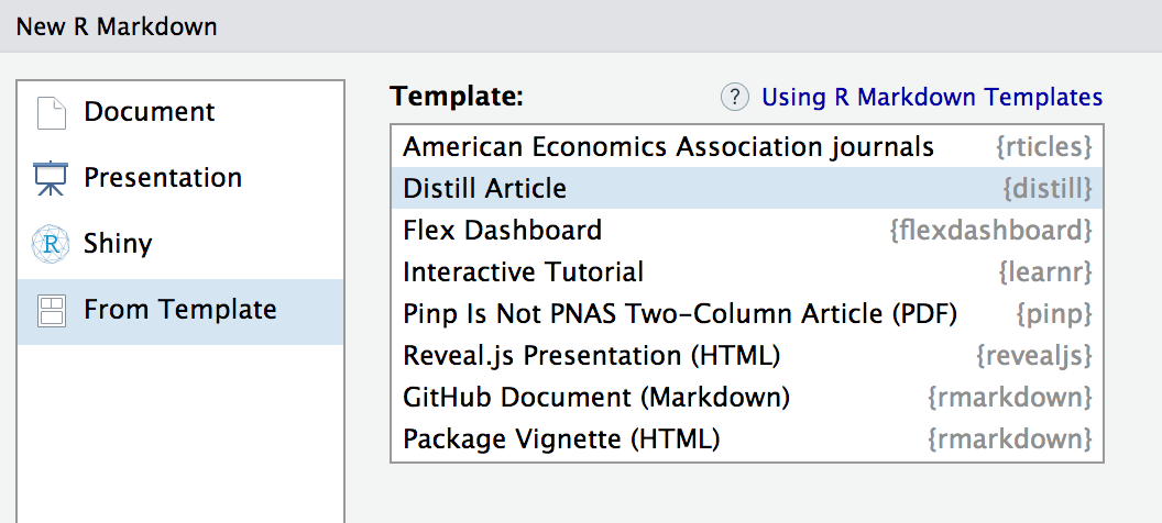
Then, go to:
From Template > Distill Article
And click on OK. The .Rmd file will be in a Distill Article format.
Distill articles use distill::distill_article as their output format, and typically include title, description, date, author/affiliation, and bibliography entries in their YAML front-matter:
description. The article’s description and author bylines are automatically rendered as part of the title area of the document.
date. The date field should be formatted as month, day, year (various notations are supported as long as the components appear in that order).
author. Author entries must have at least name and url specified (the affiliation fields are optional).
bibliography. The bibliography field is used to provide a reference to the Bibtex file where all of the sources cited in your article are defined. The citations section describes how to include references to these sources in your article.
Figures
Distill provides a number of options for laying out figures within your article. By default figures span the width of the main article body:
However, some figures benefit from using additional horizontal space. In this cases the layout chunk option enables you to specify a wide variety of other layouts.
For example, if we wanted to display a figure a bit outside the bounds of the article text, we could specify the l-body-outset layout via the layout chunk option:
```{r, layout="l-body-outset", fig.width=6, fig.height=1.5}
library(ggplot2)
ggplot(diamonds, aes(carat, price)) + geom_smooth() +
  facet_grid(~ cut)
```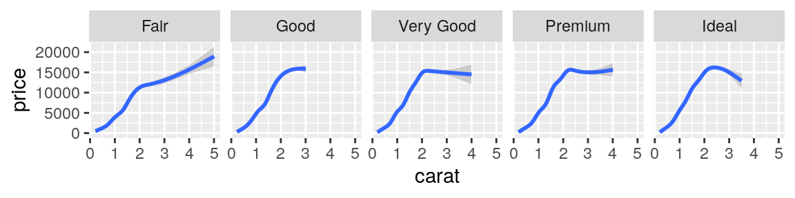
Note that when specifying an alternate layout you should also specify an appropriate fig.width and fig.height for that layout. These values don’t determine the absolute size of the figure (that’s dynamic based on the layout) but they do determine the aspect ratio of the figure.
See the documentation on figure layout for details on additional layout options.
The examples above are based on conventional R plots. Distill articles can also incorporate diagrams and interactive visualizations based on JavaScript and D3.
Tables
There are a number of options available for HTML display of data frames within Distill articles. Two options are presented to you: paged_table and kable functions.
Paged_table
Here, the paged_table() function is used to display a page-able view of the mtcars dataset built in to R:
```{r, layout="l-body-outset"}
library(rmarkdown)
paged_table(mtcars)
```
Note that layout="l-body-outset" is used to cause the table to occupy slightly more horizontal space than the article text. All of available figure layout options work as expected for tables.
See the documentation on table display for details on the various techniques available for rendering tables.
Kable
The functions used here render a Basic HTML output of kable.
```{r}
library(kableExtra)
kable(mtcars) %>%
kable_styling()
```| mpg | cyl | disp | hp | drat | wt | qsec | vs | am | gear | carb | |
|---|---|---|---|---|---|---|---|---|---|---|---|
| Mazda RX4 | 21.0 | 6 | 160.0 | 110 | 3.90 | 2.620 | 16.46 | 0 | 1 | 4 | 4 |
| Mazda RX4 Wag | 21.0 | 6 | 160.0 | 110 | 3.90 | 2.875 | 17.02 | 0 | 1 | 4 | 4 |
| Datsun 710 | 22.8 | 4 | 108.0 | 93 | 3.85 | 2.320 | 18.61 | 1 | 1 | 4 | 1 |
| Hornet 4 Drive | 21.4 | 6 | 258.0 | 110 | 3.08 | 3.215 | 19.44 | 1 | 0 | 3 | 1 |
| Hornet Sportabout | 18.7 | 8 | 360.0 | 175 | 3.15 | 3.440 | 17.02 | 0 | 0 | 3 | 2 |
| Valiant | 18.1 | 6 | 225.0 | 105 | 2.76 | 3.460 | 20.22 | 1 | 0 | 3 | 1 |
| Duster 360 | 14.3 | 8 | 360.0 | 245 | 3.21 | 3.570 | 15.84 | 0 | 0 | 3 | 4 |
| Merc 240D | 24.4 | 4 | 146.7 | 62 | 3.69 | 3.190 | 20.00 | 1 | 0 | 4 | 2 |
| Merc 230 | 22.8 | 4 | 140.8 | 95 | 3.92 | 3.150 | 22.90 | 1 | 0 | 4 | 2 |
| Merc 280 | 19.2 | 6 | 167.6 | 123 | 3.92 | 3.440 | 18.30 | 1 | 0 | 4 | 4 |
| Merc 280C | 17.8 | 6 | 167.6 | 123 | 3.92 | 3.440 | 18.90 | 1 | 0 | 4 | 4 |
| Merc 450SE | 16.4 | 8 | 275.8 | 180 | 3.07 | 4.070 | 17.40 | 0 | 0 | 3 | 3 |
| Merc 450SL | 17.3 | 8 | 275.8 | 180 | 3.07 | 3.730 | 17.60 | 0 | 0 | 3 | 3 |
| Merc 450SLC | 15.2 | 8 | 275.8 | 180 | 3.07 | 3.780 | 18.00 | 0 | 0 | 3 | 3 |
| Cadillac Fleetwood | 10.4 | 8 | 472.0 | 205 | 2.93 | 5.250 | 17.98 | 0 | 0 | 3 | 4 |
| Lincoln Continental | 10.4 | 8 | 460.0 | 215 | 3.00 | 5.424 | 17.82 | 0 | 0 | 3 | 4 |
| Chrysler Imperial | 14.7 | 8 | 440.0 | 230 | 3.23 | 5.345 | 17.42 | 0 | 0 | 3 | 4 |
| Fiat 128 | 32.4 | 4 | 78.7 | 66 | 4.08 | 2.200 | 19.47 | 1 | 1 | 4 | 1 |
| Honda Civic | 30.4 | 4 | 75.7 | 52 | 4.93 | 1.615 | 18.52 | 1 | 1 | 4 | 2 |
| Toyota Corolla | 33.9 | 4 | 71.1 | 65 | 4.22 | 1.835 | 19.90 | 1 | 1 | 4 | 1 |
| Toyota Corona | 21.5 | 4 | 120.1 | 97 | 3.70 | 2.465 | 20.01 | 1 | 0 | 3 | 1 |
| Dodge Challenger | 15.5 | 8 | 318.0 | 150 | 2.76 | 3.520 | 16.87 | 0 | 0 | 3 | 2 |
| AMC Javelin | 15.2 | 8 | 304.0 | 150 | 3.15 | 3.435 | 17.30 | 0 | 0 | 3 | 2 |
| Camaro Z28 | 13.3 | 8 | 350.0 | 245 | 3.73 | 3.840 | 15.41 | 0 | 0 | 3 | 4 |
| Pontiac Firebird | 19.2 | 8 | 400.0 | 175 | 3.08 | 3.845 | 17.05 | 0 | 0 | 3 | 2 |
| Fiat X1-9 | 27.3 | 4 | 79.0 | 66 | 4.08 | 1.935 | 18.90 | 1 | 1 | 4 | 1 |
| Porsche 914-2 | 26.0 | 4 | 120.3 | 91 | 4.43 | 2.140 | 16.70 | 0 | 1 | 5 | 2 |
| Lotus Europa | 30.4 | 4 | 95.1 | 113 | 3.77 | 1.513 | 16.90 | 1 | 1 | 5 | 2 |
| Ford Pantera L | 15.8 | 8 | 351.0 | 264 | 4.22 | 3.170 | 14.50 | 0 | 1 | 5 | 4 |
| Ferrari Dino | 19.7 | 6 | 145.0 | 175 | 3.62 | 2.770 | 15.50 | 0 | 1 | 5 | 6 |
| Maserati Bora | 15.0 | 8 | 301.0 | 335 | 3.54 | 3.570 | 14.60 | 0 | 1 | 5 | 8 |
| Volvo 142E | 21.4 | 4 | 121.0 | 109 | 4.11 | 2.780 | 18.60 | 1 | 1 | 4 | 2 |
See the documentation on cran.r to produce more complex table by learning details on HTML Table with knitr::kable and kableExtra.
Equations
Inline and display equations are supported via standard markdown MathJax syntax. You have two ways of writting it:
- The first following LaTeX math equation:
Will be rendered as:
\(\sigma = \sqrt{ \frac{1}{N} \sum_{i=1}^N (x_i -\mu)^2}\)
- The second following LaTeX math equation:
Will be rendered as:
\[ \sigma = \sqrt{ \frac{1}{N} \sum_{i=1}^N (x_i -\mu)^2} \]
Citations
Bibtex is the supported way of making academic citations. To include citations, first create a bibtex file and refer to it from the bibliography field of the YAML front-matter (as illustrated above).
For example, your bibliography file might contain:
Citations are then used in the article body with standard R Markdown notation, for example: (Allaire, Iannone, and Xie 2018) (which references an id provided in the bibliography). Note that multiple ids (separated by semicolons) can be provided.
The citation is presented inline like this: [1] (a number that displays more information on hover). If you have an appendix, a bibliography is automatically created and populated in it.
Footnotes and asides
Footnotes use standard Pandoc markdown notation, for example ^ [This will become a hover-able footnote]. The number of the footnote will be automatically generated.1
You can also optionally include notes in the gutter of the article (immediately to the right of the article text). To do this use the <aside> tag.
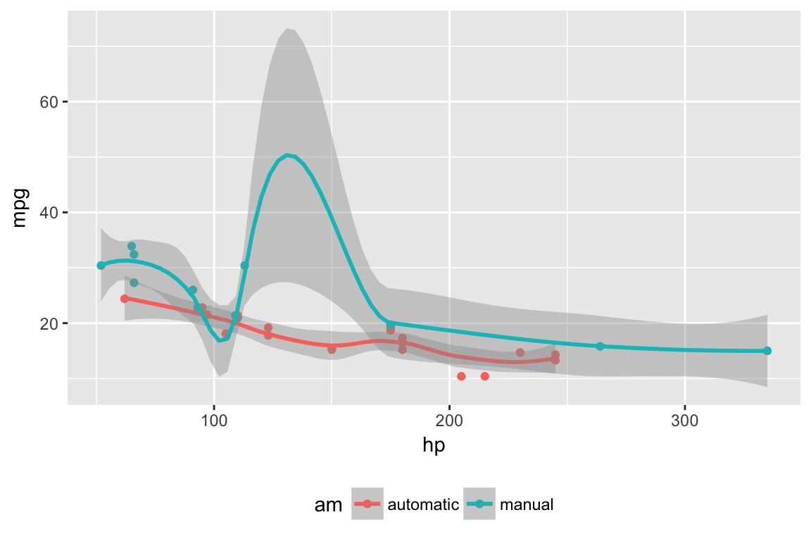
You can also include figures in the gutter. Just enclose the code chunk which generates the figure in an <aside> tag:
<aside>
```{r}
ggplot(mtcars, aes(hp, mpg)) + geom_point() + geom_smooth()
```
</aside>
Table of contents
You can add a table of contents using the toc option and specify the depth of headers that it applies to using the toc_depth option. For example:
If the table of contents depth is not explicitly specified, it defaults to 3 (meaning that all level 1, 2, and 3 headers will be included in the table of contents).
Code blocks
Syntax highlighting is provided for knitr code chunks. Note that by default the Distill format does not display the code for chunks that are evaluated to produce output (knitr option echo = FALSE).
The echo = FALSE default reflects the fact that Distill articles are often used to present the results of analyses rather than the underlying code. To display the code that was evaluated to produce output you can set the echo chunk option to TRUE:
```{r, echo=TRUE}
1 + 1
```
[1] 2To include code that is only displayed and not evaluated specify the eval=FALSE option:
```{r, eval=FALSE, echo=TRUE}
1 + 1
```
There are a number of default values that Distill establishes for knitr chunk options (these defaults also reflect the use case of presenting results/output rather than underlying code):
| Option | Value | Comment |
|---|---|---|
echo |
FALSE |
Don’t print code by default. |
warning |
FALSE |
Don’t print warnings by default. |
message |
FALSE |
Don’t print R messages by default. |
comment |
NA |
Don’t preface R output with a comment. |
R.options |
list(width = 70) |
70 character wide console output. |
Keeping R code and output at 70 characters wide (or less) is recommended for readability on a variety of devices and screen sizes.
As illustrated above, all of these defaults can be overridden on a chunk-by-chunk basis by specifying chunk options.
You can also change the global defaults using a setup chunk. For example:
```{r setup, include=FALSE}
knitr::opts_chunk$set(
  echo = TRUE,
  warning = TRUE,
  message = TRUE,
  comment = "##",
  R.options = list(width = 60)
)
```
Appendices
Appendices can be added after your article by adding the .appendix class to any level 1 or level 2 header. For example:
## Acknowledgments {.appendix}

This is a place to recognize people and institutions. It may also be a good place
to acknowledge and cite software that makes your work possible.

## Author Contributions {.appendix}

We strongly encourage you to include an author contributions statement briefly
describing what each author did.
Footnotes and references will be included in the same section, immediately beneath any custom appendices.
Allaire, J. J., Rich Iannone, and Yihui Xie. 2018. “Distill for R Markdown,” September. https://rstudio.github.io/distill.
This will become a hover-able footnote↩︎