Thierry Warin, PhD: [API] fredr: Application

Thierry Warin

doi:10.6084/m9.figshare.8870174.v2

This course will teach you how to use the fredR package.

fredR provides a complete set of R bindings to the Federal Reserve Economic Data (FRED) RESTful API, provided by the Federal Reserve Bank of St. Louis. The functions allow the user to search for and fetch time series observations as well as associated metadata within the FRED database.

Registering API key

# Load the fredR library
library(fredr)

# Enter your API key in the function "fredr_set_key"
  # fredr_set_key("abcdefghijklmnopqrstuvwxyz123456")

Before using the fredR package, you have to (freely) register to the institution.

After providing a valid email adress, you will receive an activation email. Click on it, and you will be forwarded to a control panel.

Click on the Account tab, and select API Keys. Then, click on + Request API Key.

After entering details on the use of fredR’s data, you will be provided with a unique API key.

Extracting data

# fredr_search
fredr_series_search_text(search_text = "unemployment")

# A tibble: 1,000 x 16
   id    realtime_start realtime_end title observation_sta…
   <chr> <chr>          <chr>        <chr> <chr>           
 1 UNRA… 2020-11-25     2020-11-25   Unem… 1948-01-01      
 2 UNRA… 2020-11-25     2020-11-25   Unem… 1948-01-01      
 3 LNS1… 2020-11-25     2020-11-25   Unem… 1972-01-01      
 4 NROU  2020-11-25     2020-11-25   Natu… 1949-01-01      
 5 LNU0… 2020-11-25     2020-11-25   Unem… 1972-01-01      
 6 CCSA  2020-11-25     2020-11-25   Cont… 1967-01-07      
 7 LNS1… 2020-11-25     2020-11-25   Unem… 1972-01-01      
 8 CCNSA 2020-11-25     2020-11-25   Cont… 1967-01-07      
 9 LNU0… 2020-11-25     2020-11-25   Unem… 1972-01-01      
10 UNEM… 2020-11-25     2020-11-25   Unem… 1948-01-01      
# … with 990 more rows, and 11 more variables: observation_end <chr>,
#   frequency <chr>, frequency_short <chr>, units <chr>,
#   units_short <chr>, seasonal_adjustment <chr>,
#   seasonal_adjustment_short <chr>, last_updated <chr>,
#   popularity <int>, group_popularity <int>, notes <chr>

# fredr_observations
unemployment <- fredr_series_observations(series_id = "UNRATE", 
             observation_start = as.Date("2000-01-01"),
             observation_end = as.Date("2020-01-01"))

Visualizing data

# Load the following libraries

library(dplyr)
library(ggplot2)

# Use the "Geom_line" function to create a line chart

ggplot(data = unemployment, aes(x = date, y = value)) + 
  geom_line(colour = "#f8c72d", size=1.5) +
  theme_light() +
  theme(plot.title = element_text(hjust = 0.5)) +
  labs(title = "Unemployment rate from 2000 to 2020",
       x = "Date",
       y = "percentage (%)",
       caption = "Source: Federal Reserve Bank of St. Louis")

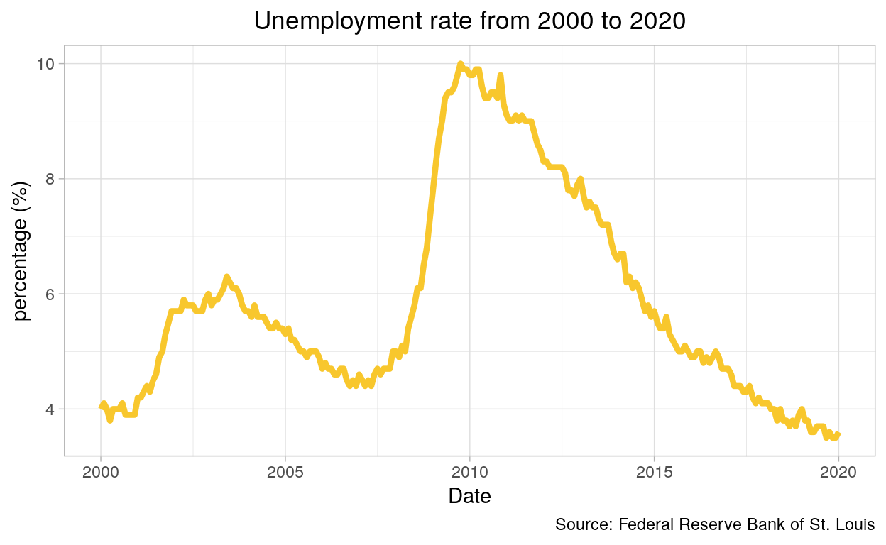
One of the most widely recognized indicators of a recession is higher unemployment rates. Looking at the graphic, we can see that around 2008-2010, the unemployment rate skyrocketed. The 2008 financial crisis was a severe worldwide economic crisis considered by many economists to have been the most serious financial crisis since the Great Depression of the 1930s.

Bitcoin Example

library(fredr)

# fredr_set_key("abcdefghijklmnopqrstuvwxyz123456") *Use your own API Key*

# fredr_search
fredr_series_search_text(search_text = "bitcoin")

# A tibble: 5 x 16
  id    realtime_start realtime_end title observation_sta…
  <chr> <chr>          <chr>        <chr> <chr>           
1 CBBT… 2020-11-25     2020-11-25   Coin… 2014-12-01      
2 CBET… 2020-11-25     2020-11-25   Coin… 2016-05-18      
3 CBBC… 2020-11-25     2020-11-25   Coin… 2017-12-20      
4 CBCC… 2020-11-25     2020-11-25   Coin… 2015-01-01      
5 CBLT… 2020-11-25     2020-11-25   Coin… 2016-08-17      
# … with 11 more variables: observation_end <chr>, frequency <chr>,
#   frequency_short <chr>, units <chr>, units_short <chr>,
#   seasonal_adjustment <chr>, seasonal_adjustment_short <chr>,
#   last_updated <chr>, popularity <int>, group_popularity <int>,
#   notes <chr>

# fredr_observations
bitcoin <- fredr_series_observations(series_id = "CBBTCUSD", 
             observation_start = as.Date("2014-01-01"),
             observation_end = as.Date("2020-01-01"))

ethereum <- fredr_series_observations(series_id = "CBETHUSD", 
             observation_start = as.Date("2014-01-01"),
             observation_end = as.Date("2020-01-01"))

litecoin <- fredr_series_observations(series_id = "CBLTCUSD", 
             observation_start = as.Date("2014-01-01"),
             observation_end = as.Date("2020-01-01"))

# Use the "bind" function to combine the three data frames together. 
#(They are already in the "gather" format so no need to manipulate the data frames further)

df_new <- bind_rows(bitcoin, ethereum)
df_final <- bind_rows(df_new, litecoin)

# Rename the Cryptocurrencies in the "series_id" column (optional)

df_final$series_id <- gsub("CBBTCUSD", "Bitcoin", df_final$series_id)
df_final$series_id <- gsub("CBETHUSD", "Ethereum", df_final$series_id)
df_final$series_id <- gsub("CBLTCUSD", "Litecoin", df_final$series_id)

library(dplyr)
library(ggplot2)

ggplot(data = df_final, aes(x = date, y = value, color = series_id)) + 
  geom_line() +
  theme_light() +
  theme(plot.title = element_text(hjust = 0.5)) +
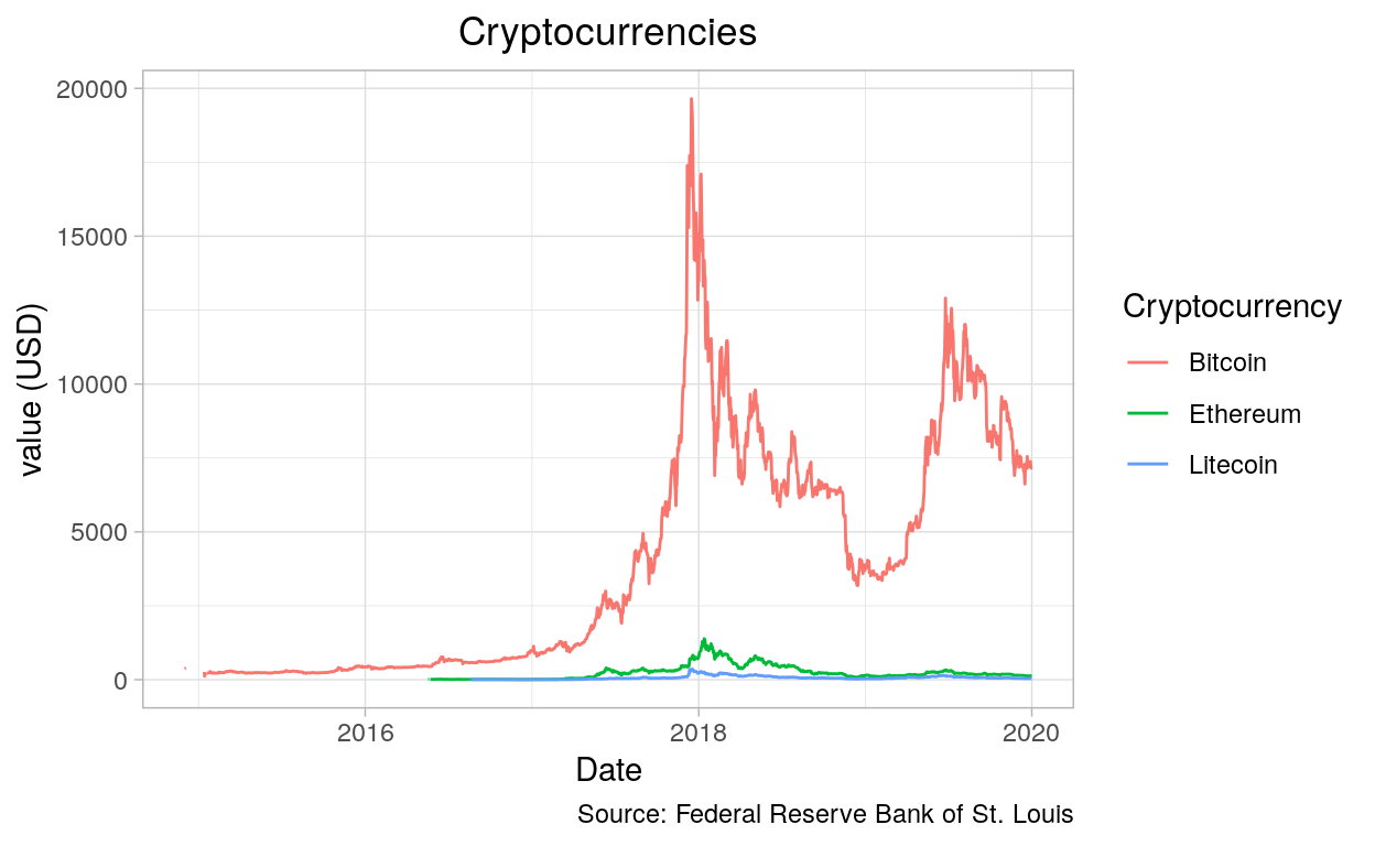
  labs(title = "Cryptocurrencies",
       x = "Date",
       y = "value (USD)",
       colour = "Cryptocurrency",
       caption = "Source: Federal Reserve Bank of St. Louis")

A more complex example

library(fredr)

# fredr_set_key("abcdefghijklmnopqrstuvwxyz123456") *Use your own API Key*

# fredr_search

internet <- fredr_series_search_text(search_text = "internet")

# fredr_observations

population_usa <- fredr_series_observations(series_id = "ITNETUSERP2USA", 
             observation_start = as.Date("2016-01-01"),
             observation_end = as.Date("2016-12-31"))

population_can <- fredr_series_observations(series_id = "ITNETUSERP2CAN", 
             observation_start = as.Date("2016-01-01"),
             observation_end = as.Date("2016-12-31"))

population_china <- fredr_series_observations(series_id = "ITNETUSERP2CHN", 
             observation_start = as.Date("2016-01-01"),
             observation_end = as.Date("2016-12-31"))

population_russia <- fredr_series_observations(series_id = "ITNETUSERP2RUS", 
             observation_start = as.Date("2016-01-01"),
             observation_end = as.Date("2016-12-31"))

# Combine all data frames together

population_usa_can <- bind_rows(population_usa, population_can)

population_usa_can_china <- bind_rows(population_usa_can, population_china)

population_usa_can_china_russia <- bind_rows(population_usa_can_china, population_russia)

population_total <- population_usa_can_china_russia

# Rename column "series_id" to "Country"
names(population_total)[names(population_total) == "series_id"] <- "Country"

# Rename each serie_id a country name

population_total$Country <- gsub("ITNETUSERP2USA", "United States of America", population_total$Country)

population_total$Country <- gsub("ITNETUSERP2CAN", "Canada", population_total$Country)

population_total$Country <- gsub("ITNETUSERP2CHN", "China", population_total$Country)

population_total$Country <- gsub("ITNETUSERP2RUS", "Russia", population_total$Country)

Visualize your data on an interactive map

library(spdep)
library(maptools)
library(leaflet)
library(dplyr)
library(maps)
library(rgdal)

map <- readOGR('world.shp')

OGR data source with driver: ESRI Shapefile 
Source: "/home/marinel/portfolio/warin/_posts/api-fredr-application/world.shp", layer: "world"
with 241 features
It has 94 fields
Integer64 fields read as strings:  POP_EST NE_ID

Shapefile link Natural Earth

# Transform factors into characters

map@data$SOVEREIGNT <- as.character(map@data$SOVEREIGNT)

# Rename Column "Country" to "SOVEREIGNT"

names(population_total)[names(population_total) == "Country"] <- "SOVEREIGNT"

# Combine data frame "population_total" with data frame "map@data"

map@data <- left_join(map@data, population_total, by = "SOVEREIGNT")

# Make sure value column is in a numeric format

map@data$value <- as.numeric(map@data$value)

# Create your labels

labels <- sprintf("<strong>%s</strong><br/>%g", map@data$SOVEREIGNT, map@data$value) %>% lapply(htmltools::HTML)

# Determinate the intervalls that will be shown in the map legend
bins <- c(50, 60, 70, 80, 90, 100)

# Choose a color scheme for your map

colors <- colorBin("YlOrRd", domain = map@data$value, bins = bins)

# Create custom icon to add to your map

internetIcon <- makeIcon(
  iconUrl = "internet.png",
  iconWidth = 20, iconHeight = 20,
  iconAnchorX = , iconAnchorY = 
)

# Plot the data using leaflet

leaflet(map) %>%
  addProviderTiles(providers$CartoDB.Positron) %>% # Basic Map
  addLegend(pal = colors, values = map@data$value, opacity = 0.7, title = NULL, position = "bottomleft") %>% # Legend
  addMarkers(lng= -106.3467712, lat= 56.1304, popup="Canada", icon = internetIcon) %>% # Canada Icon
  addMarkers(lng= -97.922211, lat= 39.381266, popup="USA", icon = internetIcon) %>% # USA Icon
  addMarkers(lng= 116.383331, lat= 39.916668, popup="China", icon = internetIcon) %>% # China Icon
  addMarkers(lng= 37.618423, lat= 55.751244, popup="Russia", icon = internetIcon) %>% # Russia Icon
  addPolygons(fillColor = ~colors(map@data$value),
              weight = 2,
              opacity = 1,
              color = "white",
              dashArray = 1,
              fillOpacity = 0.5,
              highlight = highlightOptions(weight = 2,
                                           color = "black",
                                           dashArray = 1,
                                           fillOpacity = 0.5,
                                           bringToFront = TRUE),
              label = labels
              )

Looking at the map, we can easily tell Canada and the US had the most internet users in 2016.

[API] fredr: Application

Registering API key

Extracting data

Visualizing data

Bitcoin Example

A more complex example

Citation