The comtradR package provides an R interface for the United Nations Comtrade. comtradR is a fantastic CRAN package that provides country level shipping data for a variety of commodities.
Learn how to use the comtradR package by following this example below.
Extracting Data
Search for specific countries
# Search
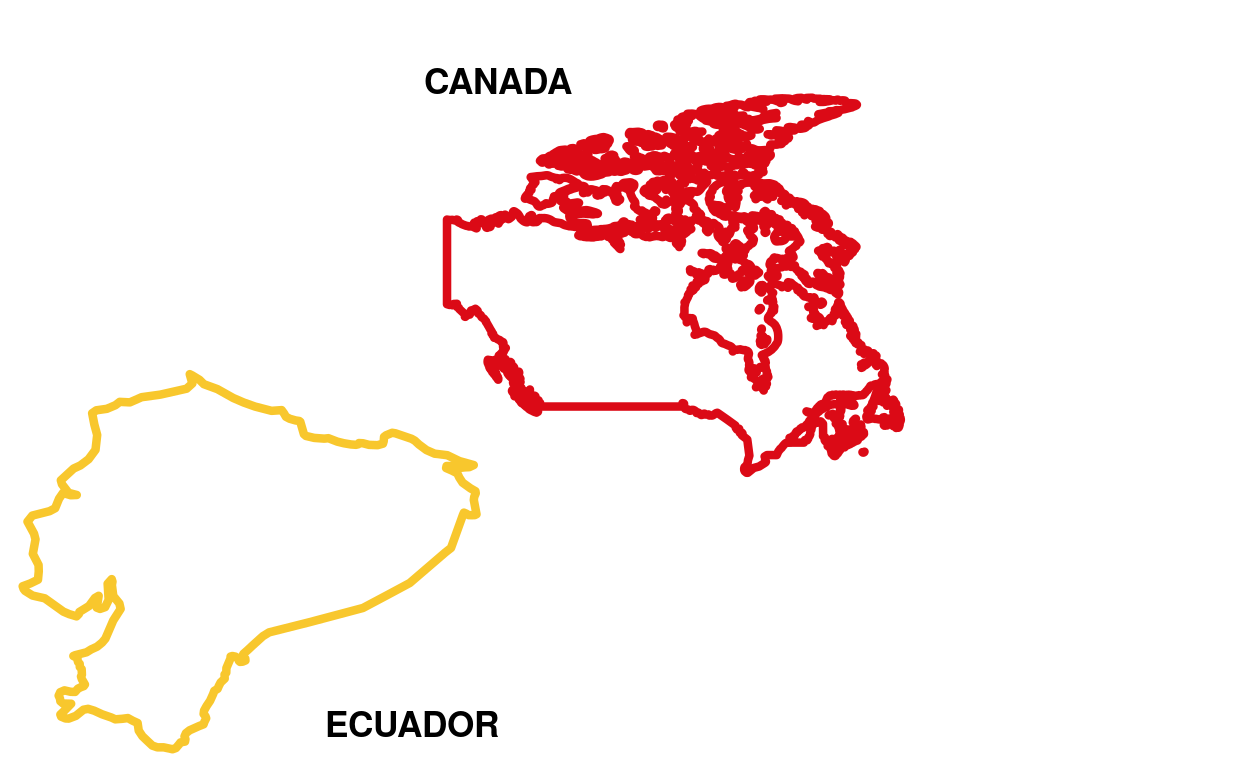
ct_country_lookup("Ecuador", "reporter")
[1] "Ecuador"ct_country_lookup(c("USA", "China", "Canada", "South Africa", "France"), "partner")
[1] "Canada" "China"
[3] "China, Hong Kong SAR" "China, Macao SAR"
[5] "France" "South Africa"
[7] "USA" "USA (before 1981)" Search for specific commodities
# Gives all the codes related to "banana"
ct_commodity_lookup("banana")
$banana
[1] "0803 - Bananas, including plantains; fresh or dried"
[2] "080300 - Fruit, edible; bananas, (including plantains), fresh or dried"
[3] "080390 - Fruit, edible; bananas, other than plantains, fresh or dried" Search for specific data
# Search data on all monthly banana exports for 2018
BananaExport <- ct_search(reporters = "Ecuador",
partners = c("All"),
trade_direction = "exports",
commod_codes = "0803",
start_date = 2018,
end_date = 2018)
str(BananaExport)
'data.frame': 75 obs. of 35 variables:
$ classification : chr "H5" "H5" "H5" "H5" ...
$ year : int 2018 2018 2018 2018 2018 2018 2018 2018 2018 2018 ...
$ period : int 2018 2018 2018 2018 2018 2018 2018 2018 2018 2018 ...
$ period_desc : chr "2018" "2018" "2018" "2018" ...
$ aggregate_level : int 4 4 4 4 4 4 4 4 4 4 ...
$ is_leaf_code : int 0 0 0 0 0 0 0 0 0 0 ...
$ trade_flow_code : int 2 2 2 2 2 2 2 2 2 2 ...
$ trade_flow : chr "Export" "Export" "Export" "Export" ...
$ reporter_code : int 218 218 218 218 218 218 218 218 218 218 ...
$ reporter : chr "Ecuador" "Ecuador" "Ecuador" "Ecuador" ...
$ reporter_iso : chr "ECU" "ECU" "ECU" "ECU" ...
$ partner_code : int 0 8 12 31 32 36 44 48 51 56 ...
$ partner : chr "World" "Albania" "Algeria" "Azerbaijan" ...
$ partner_iso : chr "WLD" "ALB" "DZA" "AZE" ...
$ second_partner_code : logi NA NA NA NA NA NA ...
$ second_partner : chr NA NA NA NA ...
$ second_partner_iso : chr NA NA NA NA ...
$ customs_proc_code : chr NA NA NA NA ...
$ customs : chr NA NA NA NA ...
$ mode_of_transport_code: chr NA NA NA NA ...
$ mode_of_transport : chr NA NA NA NA ...
$ commodity_code : chr "0803" "0803" "0803" "0803" ...
$ commodity : chr "Bananas, including plantains; fresh or dried" "Bananas, including plantains; fresh or dried" "Bananas, including plantains; fresh or dried" "Bananas, including plantains; fresh or dried" ...
$ qty_unit_code : int 8 8 8 8 8 8 8 8 8 8 ...
$ qty_unit : chr "Weight in kilograms" "Weight in kilograms" "Weight in kilograms" "Weight in kilograms" ...
$ alt_qty_unit_code : logi NA NA NA NA NA NA ...
$ alt_qty_unit : chr NA NA NA NA ...
$ qty : num 7.00e+09 3.61e+07 6.68e+07 1.57e+07 2.69e+08 ...
$ alt_qty : logi NA NA NA NA NA NA ...
$ netweight_kg : num 6.78e+09 3.21e+07 5.99e+07 1.45e+07 2.63e+08 ...
$ gross_weight_kg : logi NA NA NA NA NA NA ...
$ trade_value_usd : num 3.22e+09 1.43e+07 3.01e+07 6.71e+06 1.16e+08 ...
$ cif_trade_value_usd : logi NA NA NA NA NA NA ...
$ fob_trade_value_usd : logi NA NA NA NA NA NA ...
$ flag : int 0 0 0 0 0 0 0 0 0 0 ...
- attr(*, "url")= chr "https://comtrade.un.org/api/get?max=50000&type=C&freq=A&px=HS&ps=2018&r=218&p=all&rg=2&cc=0803&fmt=json&head=H"
- attr(*, "time_stamp")= POSIXct[1:1], format: "2020-11-25 16:09:37"
- attr(*, "req_duration")= num 1.17Data Wrangling
# Select the data you need (in this case you only need the partner and qty columns)
quantitybanana <- dplyr::select(BananaExport, partner, qty)
# Rename the "partner" column and call it "NAME" to match the "world@data" data frame
names(quantitybanana)[names(quantitybanana) == "partner"] <- "NAME"
# Rename USA and call it "United States of America" to match the "world@data" data frame
quantitybanana$NAME <- gsub("USA", "United States of America", quantitybanana$NAME)
quantitybanana$NAME <- gsub("Russian Federation", "Russia", quantitybanana$NAME)
Visualizing Data
# Use "Left join" function to combine your two data frames ("quantitybanana" and "world@data")
world@data <- left_join(world@data, quantitybanana, by = "NAME")
# Create labels
world@data$NAME <- as.character(world@data$NAME)
labels <- sprintf("<strong>%s</strong><br/>%g", world@data$NAME, world@data$qty) %>% lapply(htmltools::HTML)
# Determinate the intervalls that will be shown in the map legend
bins <- c(0, 100, 1000, 5000, 10000, 50000, 100000, 250000, 500000, 1000000, 5000000, 10000000, Inf)
# Choose a color scheme for your map
colors <- colorBin("YlOrRd", domain = world@data$qty, bins = bins)
# Create custom icon to add to your map
bananaIcon <- makeIcon(
iconUrl = "banana.png",
iconWidth = 40, iconHeight = 40,
iconAnchorX = , iconAnchorY =
)
# Plot the data using leaflet
leaflet(world) %>%
addProviderTiles(providers$CartoDB.Positron) %>%
addMarkers(lng=-78.467834, lat=-0.180653, popup="Ecuador", icon = bananaIcon) %>%
addLegend(pal = colors, values = world@data$qty, opacity = 0.7, title = NULL, position = "bottomleft") %>%
addPolygons(fillColor = ~colors(world@data$qty),
weight = 2,
opacity = 1,
color = "white",
dashArray = 1,
fillOpacity = 0.5,
highlight = highlightOptions(weight = 2,
color = "black",
dashArray = 1,
fillOpacity = 0.5,
bringToFront = TRUE),
label = labels
)
The interactive map above illustrates the quantity of bananas exported from Ecuador in 2018. The darker the color, the more bananas were exported. For reference, Ecuador exported a lot of bananas in the US, Russia, China and Canada, but very little in Australia and Mexico.
Another example
The following example shows the 2018 exports of Maple Syrup from Canada. The interactive map illustrates that Canada mostly exported Maple Syrup to the US and Australia in 2018.
library(comtradr)
library(spdep)
library(maptools)
library(leaflet)
library(dplyr)
library(maps)
library(rgdal)
ct_country_lookup("Canada", "reporter")
[1] "Canada"ct_country_lookup(c("USA", "France", "United Kingdom", "Russia"), "partner")
[1] "France" "Russian Federation" "United Kingdom"
[4] "USA" "USA (before 1981)" ct_commodity_lookup("maple syrup")
$`maple syrup`
[1] "170220 - Sugars; maple sugar, chemically pure, in solid form; maple syrup, not containing added flavouring or colouring matter"mapleSyrup <- ct_search(reporters = "Canada",
partners = c("All"),
trade_direction = "exports",
commod_codes = "170220",
start_date = 2018,
end_date = 2018)
str(mapleSyrup)
'data.frame': 64 obs. of 35 variables:
$ classification : chr "H5" "H5" "H5" "H5" ...
$ year : int 2018 2018 2018 2018 2018 2018 2018 2018 2018 2018 ...
$ period : int 2018 2018 2018 2018 2018 2018 2018 2018 2018 2018 ...
$ period_desc : chr "2018" "2018" "2018" "2018" ...
$ aggregate_level : int 6 6 6 6 6 6 6 6 6 6 ...
$ is_leaf_code : int 1 1 1 1 1 1 1 1 1 1 ...
$ trade_flow_code : int 2 2 2 2 2 2 2 2 2 2 ...
$ trade_flow : chr "Export" "Export" "Export" "Export" ...
$ reporter_code : int 124 124 124 124 124 124 124 124 124 124 ...
$ reporter : chr "Canada" "Canada" "Canada" "Canada" ...
$ reporter_iso : chr "CAN" "CAN" "CAN" "CAN" ...
$ partner_code : int 0 32 36 40 48 56 76 100 120 152 ...
$ partner : chr "World" "Argentina" "Australia" "Austria" ...
$ partner_iso : chr "WLD" "ARG" "AUS" "AUT" ...
$ second_partner_code : logi NA NA NA NA NA NA ...
$ second_partner : chr NA NA NA NA ...
$ second_partner_iso : chr NA NA NA NA ...
$ customs_proc_code : chr NA NA NA NA ...
$ customs : chr NA NA NA NA ...
$ mode_of_transport_code: chr NA NA NA NA ...
$ mode_of_transport : chr NA NA NA NA ...
$ commodity_code : chr "170220" "170220" "170220" "170220" ...
$ commodity : chr "Sugars; maple sugar, chemically pure, in solid form; maple syrup, not containing added flavouring or colouring matter" "Sugars; maple sugar, chemically pure, in solid form; maple syrup, not containing added flavouring or colouring matter" "Sugars; maple sugar, chemically pure, in solid form; maple syrup, not containing added flavouring or colouring matter" "Sugars; maple sugar, chemically pure, in solid form; maple syrup, not containing added flavouring or colouring matter" ...
$ qty_unit_code : int 8 8 8 8 8 8 8 8 8 8 ...
$ qty_unit : chr "Weight in kilograms" "Weight in kilograms" "Weight in kilograms" "Weight in kilograms" ...
$ alt_qty_unit_code : logi NA NA NA NA NA NA ...
$ alt_qty_unit : chr NA NA NA NA ...
$ qty : int 48383567 6820 2130864 44507 1467 339242 19623 10253 75 24131 ...
$ alt_qty : logi NA NA NA NA NA NA ...
$ netweight_kg : int 48383567 6820 2130864 44507 1467 339242 19623 10253 75 24131 ...
$ gross_weight_kg : logi NA NA NA NA NA NA ...
$ trade_value_usd : int 313106977 55422 13507593 356590 11739 2572061 138437 51245 569 148685 ...
$ cif_trade_value_usd : logi NA NA NA NA NA NA ...
$ fob_trade_value_usd : logi NA NA NA NA NA NA ...
$ flag : int 0 0 0 0 0 0 0 0 0 0 ...
- attr(*, "url")= chr "https://comtrade.un.org/api/get?max=50000&type=C&freq=A&px=HS&ps=2018&r=124&p=all&rg=2&cc=170220&fmt=json&head=H"
- attr(*, "time_stamp")= POSIXct[1:1], format: "2020-11-25 16:09:44"
- attr(*, "req_duration")= num 0.165quantityMaplesyrup <- dplyr::select(mapleSyrup, partner, qty)
names(quantityMaplesyrup)[names(quantityMaplesyrup) == "partner"] <- "NAME"
quantityMaplesyrup$NAME <- gsub("USA", "United States of America", quantityMaplesyrup$NAME)
quantityMaplesyrup$NAME <- gsub("Russian Federation", "Russia", quantityMaplesyrup$NAME)
world <- readOGR('world.shp')
OGR data source with driver: ESRI Shapefile
Source: "/home/marinel/portfolio/warin/_posts/api-comtradr-application/world.shp", layer: "world"
with 241 features
It has 94 fields
Integer64 fields read as strings: POP_EST NE_ID world@data$NAME <- as.character(world@data$NAME)
world@data <- left_join(world@data, quantityMaplesyrup, by = "NAME")
world@data$qty[is.na(world@data$qty)] <- 0
labels <- sprintf("<strong>%s</strong><br/>%g", world@data$NAME, world@data$qty) %>% lapply(htmltools::HTML)
bins <- c(1, 1000, 10000, 50000, 100000, 250000, 500000, 30000000, Inf)
colors <- colorBin("Reds", domain = world@data$qty, bins = bins)
mapleIcon <- makeIcon(
iconUrl = "maplesyrup.png",
iconWidth = 50, iconHeight = 50,
iconAnchorX = , iconAnchorY =
)
leaflet(world) %>%
addProviderTiles(providers$CartoDB.Positron) %>%
addMarkers(lng= -106.3467712, lat= 56.1304, popup="Canada", icon = mapleIcon) %>%
addLegend(pal = colors, values = world@data$qty, opacity = 0.7, title = NULL, position = "bottomleft") %>%
addPolygons(fillColor = ~colors(world@data$qty),
weight = 2,
opacity = 1,
color = "white",
dashArray = 1,
fillOpacity = 0.5,
highlight = highlightOptions(weight = 2,
color = "black",
dashArray = 1,
fillOpacity = 0.5,
bringToFront = TRUE),
label = labels
)