You need accurate and objective data about America’s economy? Load the bea.R package created by Andrea Batch, Jeff Chen and Walt Kampas.
The bea.R package provides an R interface for the Bureau of Economic Analysis. According to the BEA website, their mission is to promote a better understanding of the U.S. economy by providing the most timely, relevant, and accurate economic accounts data in an objective and cost-effective manner.
Learn how to use the bea.R package by following this example below :
How to use the bea.R package
You must first register for an API key from BEA by providing your name and email address. The key will be emailed to you. Once you have received your BEA API key, save it to a variable to make it easier to use later :
API Key
# Enter your beaKey number
beaKey  <- 'YOUR 36-DIGIT API KEY'
bea.R package
If you need to find a specific indicator, this following fuction allows you to search your indicator by using a keyword.
# Search the wanted indicator and its matching TableID (important for the next step)
beaSearch('personal consumption', beaKey)
      SeriesCode RowNumber                   LineDescription
   1:     DPCERL        20 Personal consumption expenditures
   2:     DPCERY        40 Personal consumption expenditures
   3:     DPCERA        20 Personal consumption expenditures
   4:     DPCERG        20 Personal consumption expenditures
   5:     DPCERC        20 Personal consumption expenditures
  ---
6066:     DCPSRC       170 Personal consumption expenditures
6067:     DCPSRX        50 Personal consumption expenditures
6068:     SWSSPY       150 Personal consumption expenditures
6069:     SWSCPY       240 Personal consumption expenditures
6070:     SWSHPY        60 Personal consumption expenditures
      LineNumber ParentLineNumber Tier  Path TableID
   1:          2                     0     2  T10101
   2:          2                     0     2  T10102
   3:          2                     0     2  T10103
   4:          2                     0     2  T10104
   5:          2                1    1   1.2  T10105
  ---
6066:         14               13    1 13.14  U90300
6067:          4                     0     4  U90300
6068:         13                     0    13  U90500
6069:         22                     0    22  U90500
6070:          4                     0     4  U90500
             DatasetName
   1:               NIPA
   2:               NIPA
   3:               NIPA
   4:               NIPA
   5:               NIPA
  ---
6066: NIUnderlyingDetail
6067: NIUnderlyingDetail
6068: NIUnderlyingDetail
6069: NIUnderlyingDetail
6070: NIUnderlyingDetail
                                                                                                                                             TableName
   1:                                                                 Table 1.1.1. Percent Change From Preceding Period in Real Gross Domestic Product
   2:                                                                      Table 1.1.2. Contributions to Percent Change in Real Gross Domestic Product
   3:                                                                                       Table 1.1.3. Real Gross Domestic Product, Quantity Indexes
   4:                                                                                            Table 1.1.4. Price Indexes for Gross Domestic Product
   5:                                                                                                              Table 1.1.5. Gross Domestic Product
  ---
6066:                                                                                   Table 9.3U. Gross Domestic Product and Final Sales of Software
6067:                                                                                   Table 9.3U. Gross Domestic Product and Final Sales of Software
6068: Table 9.5U. Contributions to Percent Change in Real Gross Domestic Product From Final Sales of Computers, Software, and Communications Equipment
6069: Table 9.5U. Contributions to Percent Change in Real Gross Domestic Product From Final Sales of Computers, Software, and Communications Equipment
6070: Table 9.5U. Contributions to Percent Change in Real Gross Domestic Product From Final Sales of Computers, Software, and Communications Equipment
              ReleaseDate     NextReleaseDate         MetaDataUpdated
   1: Feb 28 2019  8:30AM Mar 28 2019  8:30AM 2019-03-06T10:13:29.923
   2: Feb 28 2019  8:30AM Mar 28 2019  8:30AM 2019-03-06T10:13:29.923
   3: Feb 28 2019  8:30AM Mar 28 2019  8:30AM 2019-03-06T10:13:29.923
   4: Feb 28 2019  8:30AM Mar 28 2019  8:30AM 2019-03-06T10:13:29.923
   5: Feb 28 2019  8:30AM Mar 28 2019  8:30AM 2019-03-06T10:13:29.923
  ---
6066: Jul 31 2018  8:30AM Jan  1 1900 12:00AM 2019-03-06T10:13:32.840
6067: Jul 31 2018  8:30AM Jan  1 1900 12:00AM 2019-03-06T10:13:32.840
6068: Jul 31 2018  8:30AM Jan  1 1900 12:00AM 2019-03-06T10:13:32.840
6069: Jul 31 2018  8:30AM Jan  1 1900 12:00AM 2019-03-06T10:13:32.840
6070: Jul 31 2018  8:30AM Jan  1 1900 12:00AM 2019-03-06T10:13:32.840
       Account
   1: National
   2: National
   3: National
   4: National
   5: National
  ---
6066: National
6067: National
6068: National
6069: National
6070: National
                                                                                                                             apiCall
   1:               beaGet(list('UserID' = '[your_key]', 'Method' = 'GetData', 'DatasetName' = 'NIPA', 'TableName' = 'T10101', ...))
   2:               beaGet(list('UserID' = '[your_key]', 'Method' = 'GetData', 'DatasetName' = 'NIPA', 'TableName' = 'T10102', ...))
   3:               beaGet(list('UserID' = '[your_key]', 'Method' = 'GetData', 'DatasetName' = 'NIPA', 'TableName' = 'T10103', ...))
   4:               beaGet(list('UserID' = '[your_key]', 'Method' = 'GetData', 'DatasetName' = 'NIPA', 'TableName' = 'T10104', ...))
   5:               beaGet(list('UserID' = '[your_key]', 'Method' = 'GetData', 'DatasetName' = 'NIPA', 'TableName' = 'T10105', ...))
  ---
6066: beaGet(list('UserID' = '[your_key]', 'Method' = 'GetData', 'DatasetName' = 'NIUnderlyingDetail', 'TableName' = 'U90300', ...))
6067: beaGet(list('UserID' = '[your_key]', 'Method' = 'GetData', 'DatasetName' = 'NIUnderlyingDetail', 'TableName' = 'U90300', ...))
6068: beaGet(list('UserID' = '[your_key]', 'Method' = 'GetData', 'DatasetName' = 'NIUnderlyingDetail', 'TableName' = 'U90500', ...))
6069: beaGet(list('UserID' = '[your_key]', 'Method' = 'GetData', 'DatasetName' = 'NIUnderlyingDetail', 'TableName' = 'U90500', ...))
6070: beaGet(list('UserID' = '[your_key]', 'Method' = 'GetData', 'DatasetName' = 'NIUnderlyingDetail', 'TableName' = 'U90500', ...))
Extract the data
Manipulate the data
# Change your data frame from wide to long in ordrer to plot your data later
beaGather <- tidyr::gather(beaPayload, "date", "value", 8:299)

# Remove everything before a certain character (in this case we are removing everything before the underscore ("_") )
beaGather$year <- base::gsub(".*\\_","", beaGather$date)

# Add a space before every letter Q
beaGather$year <- gsub("\\s*Q\\s*", " Q", beaGather$year)

# Load the zoo package
library(zoo)

# This function is able to transform your data into the "year quarter" format.
# This is why we added a space before the letter Q, because this is the necessary format for the function to work
beaGather$year <- as.yearqtr(beaGather$year)

# Load the dplyr package
library(dplyr)
beaCFVH <- filter(beaGather, LineDescription == "Clothing and footwear" |
                             LineDescription == "Motor vehicles and parts" |
                             LineDescription == "Health care")

# This allows you to keep the years 2016 Q1 until 2019 Q4, inclusively
beaCFVH1619 <- subset(beaCFVH, year >= "2016 Q1" & year <= "2019 Q4")
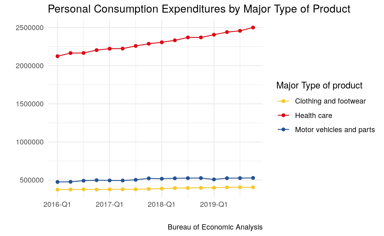
Visualize your data
palette <- c("#f8c72d", "#db0a16", "#255293")

# Plot the data using ggplot
library(ggplot2)
ggplot(data = beaCFVH1619, aes(x = year, y = value, color = LineDescription)) +
  geom_line() +
  geom_point() +
  labs (title = "Personal Consumption Expenditures by Major Type of Product",
        x = "",
        y = "",
        color = "Major Type of product",
        caption = "Bureau of Economic Analysis") +
  theme_minimal() +
  scale_color_manual(values = palette) +
  scale_x_yearqtr(format = "%Y-Q%q")
We hope this blog helped you navigate the bea.R package more easily.